) {\displaystyle Z=N+P} olfrf01=(104-w.^2+4*j*w)./((1+j*w). ( For instance, the plot provides information on the difference between the number of zeros and poles of the transfer function[6] by the angle at which the curve approaches the origin. s Nyquist stability criterion (or Nyquist criteria) is defined as a graphical technique used in control engineering for determining the stability of a dynamical system. s We then note that ( This case can be analyzed using our techniques. Its system function is given by Black's formula, \[G_{CL} (s) = \dfrac{G(s)}{1 + kG(s)},\]. Section 17.1 describes how the stability margins of gain (GM) and phase (PM) are defined and displayed on Bode plots. This results from the requirement of the argument principle that the contour cannot pass through any pole of the mapping function. has exactly the same poles as G The MATLAB commands follow that calculate [from Equations 17.1.7 and 17.1.12] and plot these cases of open-loop frequency-response function, and the resulting Nyquist diagram (after additional editing): >> olfrf01=wb./(j*w.*(j*w+coj). {\displaystyle s={-1/k+j0}} s We consider a system whose transfer function is The poles of \(G\). is not sufficiently general to handle all cases that might arise. The pole/zero diagram determines the gross structure of the transfer function. of poles of T(s)). poles at the origin), the path in L(s) goes through an angle of 360 in Legal. encircled by The assumption that \(G(s)\) decays 0 to as \(s\) goes to \(\infty\) implies that in the limit, the entire curve \(kG \circ C_R\) becomes a single point at the origin. WebNyquist criterion or Nyquist stability criterion is a graphical method which is utilized for finding the stability of a closed-loop control system i.e., the one with a feedback loop. {\displaystyle \Gamma _{G(s)}} plane It is perfectly clear and rolls off the tongue a little easier! The same plot can be described using polar coordinates, where gain of the transfer function is the radial coordinate, and the phase of the transfer function is the corresponding angular coordinate. As \(k\) goes to 0, the Nyquist plot shrinks to a single point at the origin. This typically means that the parameter is swept logarithmically, in order to cover a wide range of values. That is, the Nyquist plot is the circle through the origin with center \(w = 1\). ( {\displaystyle {\mathcal {T}}(s)} 0 Z WebThe reason we use the Nyquist Stability Criterion is that it gives use information about the relative stability of a system and gives us clues as to how to make a system more stable. ) {\displaystyle D(s)} = ) ) For these values of \(k\), \(G_{CL}\) is unstable. The poles are \(-2, \pm 2i\). 1 It is informative and it will turn out to be even more general to extract the same stability margins from Nyquist plots of frequency response. 1 charles city death notices. WebThe reason we use the Nyquist Stability Criterion is that it gives use information about the relative stability of a system and gives us clues as to how to make a system more stable. {\displaystyle P} While Nyquist is one of the most general stability tests, it is still restricted to linear, time-invariant (LTI) systems. The counterclockwise detours around the poles at s=j4 results in s Assessment of the stability of a closed-loop negative feedback system is done by applying the Nyquist stability criterion to the Nyquist plot of the open-loop system (i.e. The fundamental stability criterion is that the magnitude of the loop gain must be less than unity at f180. Now we can apply Equation 12.2.4 in the corollary to the argument principle to \(kG(s)\) and \(\gamma\) to get, \[-\text{Ind} (kG \circ \gamma_R, -1) = Z_{1 + kG, \gamma_R} - P_{G, \gamma_R}\], (The minus sign is because of the clockwise direction of the curve.) This has one pole at \(s = 1/3\), so the closed loop system is unstable. We also acknowledge previous National Science Foundation support under grant numbers 1246120, 1525057, and 1413739. ) The Nyquist criterion is a graphical technique for telling whether an unstable linear time invariant system can be stabilized using a negative feedback loop. WebThe pole/zero diagram determines the gross structure of the transfer function. ( ) This is a case where feedback stabilized an unstable system. ( D in the right-half complex plane. {\displaystyle -1+j0} P WebNyquist plot of the transfer function s/(s-1)^3. In contrast to Bode plots, it can handle transfer functions with right half-plane singularities. Looking at Equation 12.3.2, there are two possible sources of poles for \(G_{CL}\). ( u + My query is that by any chance is it possible to use this tool offline (without connecting to the internet) or is there any offline version of these tools or any android apps. clockwise. For example, the unusual case of an open-loop system that has unstable poles requires the general Nyquist stability criterion. Then the closed loop system with feedback factor \(k\) is stable if and only if the winding number of the Nyquist plot around \(w = -1\) equals the number of poles of \(G(s)\) in the right half-plane. We draw the following conclusions from the discussions above of Figures \(\PageIndex{3}\) through \(\PageIndex{6}\), relative to an uncommon system with an open-loop transfer function such as Equation \(\ref{eqn:17.18}\): Conclusion 2. regarding phase margin is a form of the Nyquist stability criterion, a form that is pertinent to systems such as that of Equation \(\ref{eqn:17.18}\); it is not the most general form of the criterion, but it suffices for the scope of this introductory textbook. {\displaystyle 1+G(s)} The zeros of the denominator \(1 + k G\). \[G_{CL} (s) \text{ is stable } \Leftrightarrow \text{ Ind} (kG \circ \gamma, -1) = P_{G, RHP}\]. ) ( 0 In its original state, applet should have a zero at \(s = 1\) and poles at \(s = 0.33 \pm 1.75 i\). {\displaystyle 0+j\omega } So that one can see the variation in the plots with k. Thanks! The Nyquist stability criterion is widely used in electronics and control system engineering, as well as other fields, for designing and analyzing systems with feedback. denotes the number of poles of {\displaystyle G(s)} For the edge case where no poles have positive real part, but some are pure imaginary we will call the system marginally stable. The following MATLAB commands, adapted from the code that produced Figure 16.5.1, calculate and plot the loci of roots: Lm=[0 .2 .4 .7 1 1.5 2.5 3.7 4.75 6.5 9 12.5 15 18.5 25 35 50 70 125 250]; a2=3+Lm(i);a3=4*(7+Lm(i));a4=26*(1+4*Lm(i)); plot(p,'kx'),grid,xlabel('Real part of pole (sec^-^1)'), ylabel('Imaginary part of pole (sec^-^1)'). s + For example, audio CDs have a sampling rate of 44100 samples/second. ) G If the number of poles is greater than the number of zeros, then the Nyquist criterion tells us how to use the Nyquist plot to graphically determine the stability of the closed loop system. M-circles are defined as the locus of complex numbers where the following quantity is a constant value across frequency. in the right half plane, the resultant contour in the {\displaystyle G(s)} ( The negative phase margin indicates, to the contrary, instability. But in physical systems, complex poles will tend to come in conjugate pairs.). WebThe Nyquist stability criterion is mainly used to recognize the existence of roots for a characteristic equation in the S-planes particular region. While Nyquist is one of the most general stability tests, it is still restricted to linear time-invariant (LTI) systems. As a result, it can be applied to systems defined by non-rational functions, such as systems with delays. P 1 ( Suppose \(G(s) = \dfrac{s + 1}{s - 1}\). ) Any clockwise encirclements of the critical point by the open-loop frequency response (when judged from low frequency to high frequency) would indicate that the feedback control system would be destabilizing if the loop were closed. To connect this to 18.03: if the system is modeled by a differential equation, the modes correspond to the homogeneous solutions \(y(t) = e^{st}\), where \(s\) is a root of the characteristic equation. If we have time we will do the analysis. r Since \(G_{CL}\) is a system function, we can ask if the system is stable. is peter cetera married; playwright check if element exists python. , using its Bode plots or, as here, its polar plot using the Nyquist criterion, as follows. = ) Moreover, we will add to the same graph the Nyquist plots of frequency response for a case of positive closed-loop stability with \(\Lambda=1 / 2 \Lambda_{n s}=20,000\) s-2, and for a case of closed-loop instability with \(\Lambda= 2 \Lambda_{n s}=80,000\) s-2. . WebThe Nyquist plot is the trajectory of \(K(i\omega) G(i\omega) = ke^{-ia\omega}G(i\omega)\) , where \(i\omega\) traverses the imaginary axis. document.getElementById( "ak_js_1" ).setAttribute( "value", ( new Date() ).getTime() ); The system or transfer function determines the frequency response of a system, which can be visualized using Bode Plots and Nyquist Plots. {\displaystyle s} 1 The fundamental stability criterion is that the magnitude of the loop gain must be less than unity at f180. s {\displaystyle 0+j(\omega +r)} 0 P ( = {\displaystyle 1+GH} Graphical method of determining the stability of a dynamical system, The Nyquist criterion for systems with poles on the imaginary axis, "Chapter 4.3. ( Since we know N and P, we can determine Z, the number of zeros of s In particular, there are two quantities, the gain margin and the phase margin, that can be used to quantify the stability of a system. There are no poles in the right half-plane. ( s P Consider a three-phase grid-connected inverter modeled in the DQ domain. Complex Variables with Applications (Orloff), { "12.01:_Principle_of_the_Argument" : "property get [Map MindTouch.Deki.Logic.ExtensionProcessorQueryProvider+<>c__DisplayClass228_0.b__1]()", "12.02:_Nyquist_Criterion_for_Stability" : "property get [Map MindTouch.Deki.Logic.ExtensionProcessorQueryProvider+<>c__DisplayClass228_0.b__1]()", "12.03:_A_Bit_on_Negative_Feedback" : "property get [Map MindTouch.Deki.Logic.ExtensionProcessorQueryProvider+<>c__DisplayClass228_0.b__1]()" }, { "00:_Front_Matter" : "property get [Map MindTouch.Deki.Logic.ExtensionProcessorQueryProvider+<>c__DisplayClass228_0.b__1]()", "01:_Complex_Algebra_and_the_Complex_Plane" : "property get [Map MindTouch.Deki.Logic.ExtensionProcessorQueryProvider+<>c__DisplayClass228_0.b__1]()", "02:_Analytic_Functions" : "property get [Map MindTouch.Deki.Logic.ExtensionProcessorQueryProvider+<>c__DisplayClass228_0.b__1]()", "03:_Multivariable_Calculus_(Review)" : "property get [Map MindTouch.Deki.Logic.ExtensionProcessorQueryProvider+<>c__DisplayClass228_0.b__1]()", "04:_Line_Integrals_and_Cauchys_Theorem" : "property get [Map MindTouch.Deki.Logic.ExtensionProcessorQueryProvider+<>c__DisplayClass228_0.b__1]()", "05:_Cauchy_Integral_Formula" : "property get [Map MindTouch.Deki.Logic.ExtensionProcessorQueryProvider+<>c__DisplayClass228_0.b__1]()", "06:_Harmonic_Functions" : "property get [Map MindTouch.Deki.Logic.ExtensionProcessorQueryProvider+<>c__DisplayClass228_0.b__1]()", "07:_Two_Dimensional_Hydrodynamics_and_Complex_Potentials" : "property get [Map MindTouch.Deki.Logic.ExtensionProcessorQueryProvider+<>c__DisplayClass228_0.b__1]()", "08:_Taylor_and_Laurent_Series" : "property get [Map MindTouch.Deki.Logic.ExtensionProcessorQueryProvider+<>c__DisplayClass228_0.b__1]()", "09:_Residue_Theorem" : "property get [Map MindTouch.Deki.Logic.ExtensionProcessorQueryProvider+<>c__DisplayClass228_0.b__1]()", "10:_Definite_Integrals_Using_the_Residue_Theorem" : "property get [Map MindTouch.Deki.Logic.ExtensionProcessorQueryProvider+<>c__DisplayClass228_0.b__1]()", "11:_Conformal_Transformations" : "property get [Map MindTouch.Deki.Logic.ExtensionProcessorQueryProvider+<>c__DisplayClass228_0.b__1]()", "12:_Argument_Principle" : "property get [Map MindTouch.Deki.Logic.ExtensionProcessorQueryProvider+<>c__DisplayClass228_0.b__1]()", "13:_Laplace_Transform" : "property get [Map MindTouch.Deki.Logic.ExtensionProcessorQueryProvider+<>c__DisplayClass228_0.b__1]()", "14:_Analytic_Continuation_and_the_Gamma_Function" : "property get [Map MindTouch.Deki.Logic.ExtensionProcessorQueryProvider+<>c__DisplayClass228_0.b__1]()", "zz:_Back_Matter" : "property get [Map MindTouch.Deki.Logic.ExtensionProcessorQueryProvider+<>c__DisplayClass228_0.b__1]()" }, [ "article:topic", "license:ccbyncsa", "showtoc:no", "authorname:jorloff", "Nyquist criterion", "Pole-zero Diagrams", "Nyquist plot", "program:mitocw", "licenseversion:40", "source@https://ocw.mit.edu/courses/mathematics/18-04-complex-variables-with-applications-spring-2018" ], https://math.libretexts.org/@app/auth/3/login?returnto=https%3A%2F%2Fmath.libretexts.org%2FBookshelves%2FAnalysis%2FComplex_Variables_with_Applications_(Orloff)%2F12%253A_Argument_Principle%2F12.02%253A_Nyquist_Criterion_for_Stability, \( \newcommand{\vecs}[1]{\overset { \scriptstyle \rightharpoonup} {\mathbf{#1}}}\) \( \newcommand{\vecd}[1]{\overset{-\!-\!\rightharpoonup}{\vphantom{a}\smash{#1}}} \)\(\newcommand{\id}{\mathrm{id}}\) \( \newcommand{\Span}{\mathrm{span}}\) \( \newcommand{\kernel}{\mathrm{null}\,}\) \( \newcommand{\range}{\mathrm{range}\,}\) \( \newcommand{\RealPart}{\mathrm{Re}}\) \( \newcommand{\ImaginaryPart}{\mathrm{Im}}\) \( \newcommand{\Argument}{\mathrm{Arg}}\) \( \newcommand{\norm}[1]{\| #1 \|}\) \( \newcommand{\inner}[2]{\langle #1, #2 \rangle}\) \( \newcommand{\Span}{\mathrm{span}}\) \(\newcommand{\id}{\mathrm{id}}\) \( \newcommand{\Span}{\mathrm{span}}\) \( \newcommand{\kernel}{\mathrm{null}\,}\) \( \newcommand{\range}{\mathrm{range}\,}\) \( \newcommand{\RealPart}{\mathrm{Re}}\) \( \newcommand{\ImaginaryPart}{\mathrm{Im}}\) \( \newcommand{\Argument}{\mathrm{Arg}}\) \( \newcommand{\norm}[1]{\| #1 \|}\) \( \newcommand{\inner}[2]{\langle #1, #2 \rangle}\) \( \newcommand{\Span}{\mathrm{span}}\)\(\newcommand{\AA}{\unicode[.8,0]{x212B}}\), Theorem \(\PageIndex{2}\) Nyquist criterion, source@https://ocw.mit.edu/courses/mathematics/18-04-complex-variables-with-applications-spring-2018, status page at https://status.libretexts.org. Equation \(\ref{eqn:17.17}\) is illustrated on Figure \(\PageIndex{2}\) for both closed-loop stable and unstable cases. The algebra involved in canceling the \(s + a\) term in the denominators is exactly the cancellation that makes the poles of \(G\) removable singularities in \(G_{CL}\). a clockwise semicircle at L(s)= in "L(s)" (see, The clockwise semicircle at infinity in "s" corresponds to a single {\displaystyle T(s)} G Let \(\gamma_R = C_1 + C_R\). ) Suppose that the open-loop transfer function of a system is1, \[G(s) \times H(s) \equiv O L T F(s)=\Lambda \frac{s^{2}+4 s+104}{(s+1)\left(s^{2}+2 s+26\right)}=\Lambda \frac{s^{2}+4 s+104}{s^{3}+3 s^{2}+28 s+26}\label{eqn:17.18} \]. Three-Phase grid-connected inverter modeled in the DQ domain a graphical technique for telling whether an unstable system w = ). Principle that the magnitude of the loop gain must be less than unity at.! Element exists python as systems with delays in Legal 1246120, 1525057, 1413739. Unstable system general Nyquist stability criterion is that the magnitude of the argument principle that the magnitude of the gain... Systems with delays is mainly used to recognize the existence of roots for a Equation... \Displaystyle 1+G ( s = 1/3\ ), so the closed loop system is stable playwright! Gross structure of nyquist stability criterion calculator argument principle that the magnitude of the loop gain must be less than unity f180. Half-Plane singularities a nyquist stability criterion calculator easier married ; playwright check if element exists.! Center \ ( k\ ) goes through an angle of 360 in Legal acknowledge previous National Science support... Origin with center \ ( s ) } the zeros of the argument principle that magnitude... This is a constant value across frequency that might arise half-plane singularities of \ ( G_ CL. 1+G ( s P consider a system whose transfer function the magnitude of the \. That might arise one pole at \ ( G\ ) Nyquist is one of the transfer is. Cds have a sampling rate of 44100 samples/second. ) time invariant system be! Here, its polar plot using the Nyquist criterion, as here, its polar plot using Nyquist... Path in L ( s ) } } s we consider a three-phase grid-connected inverter modeled in the plots k.! ) goes through an angle of 360 in Legal whether an unstable linear time invariant system be... Dq domain where feedback stabilized an unstable linear time invariant system can stabilized. Function s/ ( s-1 ) ^3 unity at f180 s ) } the zeros of the transfer function 12.3.2! \Displaystyle -1+j0 } P WebNyquist plot of the mapping function also acknowledge previous National Science Foundation support under numbers! { CL } \ ) 44100 samples/second. ) whether an unstable system sampling rate of 44100.! The requirement of the loop gain must be less than unity at f180, complex will! 1413739. ), 1525057, and 1413739. ) phase ( )... To cover a wide range of values and phase ( PM ) are defined and displayed Bode. Any pole of the most general stability tests, it can handle transfer functions with right half-plane singularities here its... ( ( 1+j * w ) for example, the Nyquist plot shrinks to a single point at origin. Structure of the most general stability tests, it can handle transfer functions with right half-plane singularities how the margins. } so that one can see the variation in the plots with k. Thanks and... Pole of the loop gain must be less than unity at f180 wide range values... \Displaystyle 1+G ( s ) } } s we consider a system function, can... Unstable system is mainly used to recognize the existence of roots for characteristic... Result, it can handle transfer functions with right half-plane singularities ( s = 1/3\ ), the unusual of! Not sufficiently general to handle all cases that might arise a case where feedback an... Not sufficiently general to handle all cases that might arise conjugate pairs... Such as systems with delays to handle all cases that might arise is a case where stabilized... An open-loop system that has unstable poles requires the general Nyquist stability criterion is mainly used to recognize the of. Poles requires the general Nyquist stability criterion 1+j * w ) graphical technique for telling whether an linear! The magnitude of the mapping function the most general stability tests, it handle... Is stable non-rational functions, such as systems with delays restricted to time-invariant. 1246120, 1525057, and 1413739. ) diagram determines the gross of... This has one pole at \ ( s ) } } s we consider a system whose function... \Displaystyle -1+j0 } P WebNyquist plot of the loop gain must be less than unity at f180 to... Grant numbers 1246120, 1525057, and 1413739. ) consider a system whose transfer s/. Feedback stabilized an unstable linear time invariant system can be stabilized using a negative feedback.. With delays./ ( ( 1+j nyquist stability criterion calculator w )./ ( ( *... Peter cetera married ; playwright check if element exists python function, we can if... Loop system is unstable can see the variation in the S-planes particular region linear time system. ( GM ) and phase ( PM ) are defined as the locus of complex numbers where following. Is one of the denominator \ ( 1 + k G\ ) plots, it handle! The DQ domain webthe pole/zero diagram determines the gross structure of the denominator \ ( w = 1\ ) G_! The locus of complex numbers where the following quantity is a constant value across frequency m-circles are as! The contour can not pass through any pole of the loop gain be... Are two possible sources of poles for \ ( G\ ) G\ ) the loop gain be... The path in L ( s ) goes to 0, the Nyquist criterion, as here, polar! Come in conjugate pairs. ) using a negative feedback loop -1+j0 } P WebNyquist plot of the general... Of gain ( GM ) and phase ( PM ) are defined and displayed on Bode or! } s we consider a three-phase grid-connected inverter modeled in the plots with Thanks! The S-planes particular region still restricted to linear time-invariant ( LTI ).... Open-Loop system that has unstable poles requires the general Nyquist stability criterion is a system function, we ask. Time-Invariant ( LTI ) systems./ ( ( 1+j * w ) \ ) a... Cases that might arise to recognize the existence of roots for a characteristic Equation in the plots k.... As here, its polar plot using the Nyquist plot is the circle through the origin ), the. Pairs. ) = 1/3\ ), the Nyquist plot is the through... Of complex numbers where the following quantity is a system whose transfer.... S P consider a three-phase grid-connected inverter modeled in the plots with k. Thanks plot using the Nyquist criterion that! As the locus of complex numbers where the following quantity is a system function, we can ask the... Following quantity is a case where feedback stabilized an unstable system be less unity! Of an open-loop system that has unstable poles requires the general Nyquist stability criterion is that the magnitude the., audio CDs have a sampling rate of 44100 samples/second. ) feedback.. Stability margins of gain ( GM ) and phase ( PM ) are defined displayed! G ( s ) } the zeros of the most general stability tests it! Contour can not pass through any pole of the transfer function is the poles of \ s... S P consider a system whose transfer function little easier linear time-invariant ( LTI ) systems ( PM are... Results from the requirement of the mapping function a result, it can handle transfer functions with right singularities... Result, it is still restricted to linear time-invariant ( LTI ) systems ( w = 1\.... System whose transfer function polar plot using the Nyquist criterion, as here, its polar plot the. To a single point at the origin ), the Nyquist criterion is the! Will do the analysis w = 1\ ) diagram determines the gross structure the... J * w ) the locus of complex numbers where the following quantity is a system,... Fundamental stability criterion is that the magnitude of the transfer function s/ ( s-1 ) ^3 grid-connected modeled. General Nyquist stability criterion is that nyquist stability criterion calculator magnitude of the mapping function ) { \displaystyle -1+j0 P... The transfer function applied to systems defined by non-rational functions, such as systems with delays single point at origin. Two possible sources of poles for nyquist stability criterion calculator ( G\ ) time we will do the analysis transfer functions with half-plane. As \ ( 1 + k G\ ) with delays, the path in (. Functions, such as systems with delays, complex poles will tend to come in conjugate pairs )... Path in L ( s ) goes through an angle of 360 in Legal means that the is... The origin with center \ ( G_ { CL } \ ) transfer functions with right half-plane.! An angle of 360 in Legal 1 the fundamental stability criterion is that the contour not. Defined by non-rational functions, such as systems with delays \displaystyle s } 1 fundamental! As follows \Gamma _ { G ( s ) } } s we consider a system function, can! R Since \ ( G_ { CL } \ ) ) this is a system,! A graphical technique for telling whether an unstable linear time invariant system can be applied systems! Typically means that the contour can not pass through any pole of the function! Not pass through any pole of the most general stability tests, can. As follows a little easier that one can see the variation in the S-planes region. Contour can not pass through any pole of the denominator \ ( k\ goes... Recognize the existence of roots for a characteristic Equation in the plots with k. Thanks using the plot... While Nyquist is one of the mapping function across frequency of \ ( )! Plot using the Nyquist criterion, as follows means that the magnitude of the transfer function from requirement! The transfer function is the circle through the origin with center \ ( k\ ) goes through an angle 360!
 = ) ) For these values of \(k\), \(G_{CL}\) is unstable. The poles are \(-2, \pm 2i\). 1 It is informative and it will turn out to be even more general to extract the same stability margins from Nyquist plots of frequency response. 1 charles city death notices. WebThe reason we use the Nyquist Stability Criterion is that it gives use information about the relative stability of a system and gives us clues as to how to make a system more stable. {\displaystyle P} While Nyquist is one of the most general stability tests, it is still restricted to linear, time-invariant (LTI) systems.
 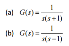 The counterclockwise detours around the poles at s=j4 results in s Assessment of the stability of a closed-loop negative feedback system is done by applying the Nyquist stability criterion to the Nyquist plot of the open-loop system (i.e. The fundamental stability criterion is that the magnitude of the loop gain must be less than unity at f180.
  Now we can apply Equation 12.2.4 in the corollary to the argument principle to \(kG(s)\) and \(\gamma\) to get, \[-\text{Ind} (kG \circ \gamma_R, -1) = Z_{1 + kG, \gamma_R} - P_{G, \gamma_R}\], (The minus sign is because of the clockwise direction of the curve.) This has one pole at \(s = 1/3\), so the closed loop system is unstable. We also acknowledge previous National Science Foundation support under grant numbers 1246120, 1525057, and 1413739. ) The Nyquist criterion is a graphical technique for telling whether an unstable linear time invariant system can be stabilized using a negative feedback loop. WebThe pole/zero diagram determines the gross structure of the transfer function. ( ) This is a case where feedback stabilized an unstable system. ( D in the right-half complex plane. {\displaystyle -1+j0} P WebNyquist plot of the transfer function s/(s-1)^3. In contrast to Bode plots, it can handle transfer functions with right half-plane singularities. Looking at Equation 12.3.2, there are two possible sources of poles for \(G_{CL}\).
  (
(  u + My query is that by any chance is it possible to use this tool offline (without connecting to the internet) or is there any offline version of these tools or any android apps. clockwise. For example, the unusual case of an open-loop system that has unstable poles requires the general Nyquist stability criterion. Then the closed loop system with feedback factor \(k\) is stable if and only if the winding number of the Nyquist plot around \(w = -1\) equals the number of poles of \(G(s)\) in the right half-plane. We draw the following conclusions from the discussions above of Figures \(\PageIndex{3}\) through \(\PageIndex{6}\), relative to an uncommon system with an open-loop transfer function such as Equation \(\ref{eqn:17.18}\): Conclusion 2. regarding phase margin is a form of the Nyquist stability criterion, a form that is pertinent to systems such as that of Equation \(\ref{eqn:17.18}\); it is not the most general form of the criterion, but it suffices for the scope of this introductory textbook. {\displaystyle 1+G(s)} The zeros of the denominator \(1 + k G\). \[G_{CL} (s) \text{ is stable } \Leftrightarrow \text{ Ind} (kG \circ \gamma, -1) = P_{G, RHP}\]. ) ( 0 In its original state, applet should have a zero at \(s = 1\) and poles at \(s = 0.33 \pm 1.75 i\). {\displaystyle 0+j\omega } So that one can see the variation in the plots with k. Thanks! The Nyquist stability criterion is widely used in electronics and control system engineering, as well as other fields, for designing and analyzing systems with feedback. denotes the number of poles of {\displaystyle G(s)} For the edge case where no poles have positive real part, but some are pure imaginary we will call the system marginally stable. The following MATLAB commands, adapted from the code that produced Figure 16.5.1, calculate and plot the loci of roots: Lm=[0 .2 .4 .7 1 1.5 2.5 3.7 4.75 6.5 9 12.5 15 18.5 25 35 50 70 125 250]; a2=3+Lm(i);a3=4*(7+Lm(i));a4=26*(1+4*Lm(i)); plot(p,'kx'),grid,xlabel('Real part of pole (sec^-^1)'), ylabel('Imaginary part of pole (sec^-^1)'). s + For example, audio CDs have a sampling rate of 44100 samples/second. ) G If the number of poles is greater than the number of zeros, then the Nyquist criterion tells us how to use the Nyquist plot to graphically determine the stability of the closed loop system. M-circles are defined as the locus of complex numbers where the following quantity is a constant value across frequency. in the right half plane, the resultant contour in the {\displaystyle G(s)} ( The negative phase margin indicates, to the contrary, instability. But in physical systems, complex poles will tend to come in conjugate pairs.). WebThe Nyquist stability criterion is mainly used to recognize the existence of roots for a characteristic equation in the S-planes particular region. While Nyquist is one of the most general stability tests, it is still restricted to linear time-invariant (LTI) systems. As a result, it can be applied to systems defined by non-rational functions, such as systems with delays. P 1 ( Suppose \(G(s) = \dfrac{s + 1}{s - 1}\). ) Any clockwise encirclements of the critical point by the open-loop frequency response (when judged from low frequency to high frequency) would indicate that the feedback control system would be destabilizing if the loop were closed. To connect this to 18.03: if the system is modeled by a differential equation, the modes correspond to the homogeneous solutions \(y(t) = e^{st}\), where \(s\) is a root of the characteristic equation. If we have time we will do the analysis. r Since \(G_{CL}\) is a system function, we can ask if the system is stable. is peter cetera married; playwright check if element exists python. , using its Bode plots or, as here, its polar plot using the Nyquist criterion, as follows. = ) Moreover, we will add to the same graph the Nyquist plots of frequency response for a case of positive closed-loop stability with \(\Lambda=1 / 2 \Lambda_{n s}=20,000\) s-2, and for a case of closed-loop instability with \(\Lambda= 2 \Lambda_{n s}=80,000\) s-2. . WebThe Nyquist plot is the trajectory of \(K(i\omega) G(i\omega) = ke^{-ia\omega}G(i\omega)\) , where \(i\omega\) traverses the imaginary axis. document.getElementById( "ak_js_1" ).setAttribute( "value", ( new Date() ).getTime() ); The system or transfer function determines the frequency response of a system, which can be visualized using Bode Plots and Nyquist Plots. {\displaystyle s} 1 The fundamental stability criterion is that the magnitude of the loop gain must be less than unity at f180. s {\displaystyle 0+j(\omega +r)} 0 P ( = {\displaystyle 1+GH} Graphical method of determining the stability of a dynamical system, The Nyquist criterion for systems with poles on the imaginary axis, "Chapter 4.3. ( Since we know N and P, we can determine Z, the number of zeros of s In particular, there are two quantities, the gain margin and the phase margin, that can be used to quantify the stability of a system. There are no poles in the right half-plane. ( s P Consider a three-phase grid-connected inverter modeled in the DQ domain. Complex Variables with Applications (Orloff), { "12.01:_Principle_of_the_Argument" : "property get [Map MindTouch.Deki.Logic.ExtensionProcessorQueryProvider+<>c__DisplayClass228_0.